4 Dates and times: lubridate
Resources:
Suggested data set: weather-kiel-holtenau
4.1 What is Lubridate?
Lubridate is an R-Package designed to ease working with date/time variables. These can be challenging in baseR and lubridate allows for frictionless working with dates and times, hence the name.
Lubridate ist part of the tidyverse package, but can be installed seperately as well. It probably reveals most of its usefullness in collaboration with other tidyverse packages. A useful extension, depending on your data, might be the time-series package which is not part of tidyverse.
All mentioned packages can be optained with the following commands in the RStudio console.
install.packages(“lubridate”) install.packages(“tidyverse”) install.packages(“testit”)
If they have been installed previously in your environment, they might have to be called upon by using library(tidyverse) and so forth - see code chunks below.
4.2 Basics
Some examples of real world date-time formats found in datasets:
How people talk about dates and times often differs from the notation. Depending on the specific use of the data, the given information might be more or less granular. When people in the USA talk distance between two places, they often give an approximation of how long it will take a person to drive from A to B and round-up or down to the hour.
Flight schedules will most likely be exact to the minute, while some sensordata will probably need to be exact to the second. So there will be differing granularity in date and time data.
Even if this would not be challenging, we still would have to deal with different notations of date and time. People in Germany will write a day-date like: dd.mm.yyyy or short dd.mm.yy, while the anglo-saxon realm will use mm.dd.yyyy frequently and the most chronologically sound way would be to use yyyy.mm.dd, but this doesn’t seem to stick with humans.
On top of these issues there’s the fact that time itself does not make the impression of being the most exact parameter out there. Physical time might appear linear, but the way our planet revolves within our galaxy has made it neccessary to adjust date and times every now and then, so our calendar stays in tune with defined periods and seasons. This creates leap years, skipped seconds, daylight-savings time and last, but not least time-zones, which can mess things up even further. After defining date-time data as distinct “places in time” often the need for calculation with them arises.
4.3 Import data, clean date-time
We will apply the lubridate package to Weather data from on stationary sensor in northern Germany, the weather station in Kiel-Holtenau to be more exact.
Before we introduce the library, the technical prerequisites must be created.
library(readr)          # part of the tidyverse
library(lubridate)      # the mentioned lubrication for date-time wrangling
##
## Attache Paket: 'lubridate'## The following object is masked from 'package:base':
##
## date## -- Attaching packages ---------------## v ggplot2 3.3.0 v purrr 0.3.2
## v tibble 3.0.0 v dplyr 0.8.5
## v tidyr 1.0.0 v stringr 1.4.0
## v ggplot2 3.3.0 v forcats 0.5.0## Warning: Paket 'ggplot2' wurde unter R Version 3.6.3 erstellt## Warning: Paket 'tibble' wurde unter R Version 3.6.3 erstellt## Warning: Paket 'dplyr' wurde unter R Version 3.6.3 erstellt## Warning: Paket 'forcats' wurde unter R Version 3.6.3 erstellt## -- Conflicts ------------------------
## x lubridate::as.difftime() masks base::as.difftime()
## x lubridate::date() masks base::date()
## x dplyr::filter() masks stats::filter()
## x lubridate::intersect() masks base::intersect()
## x dplyr::lag() masks stats::lag()
## x lubridate::setdiff() masks base::setdiff()
## x lubridate::union() masks base::union()library(ggplot2) # data visualisation package (is actually part of tidyverse, but still)
library(testit) # testing data selections## Warning: Paket 'testit' wurde unter R Version 3.6.3 erstelltWith the lubridate package activated, we can now call some simple functions to check where we are in time:
## [1] "2020-05-08"## [1] "2020-05-08 07:42:46 CEST"## [1] "2020-05-08"## [1] "2020-05-08 07:42:46 CEST"## [1] "Europe/Berlin"The first function delivers a date, while the second delivers a date-time (a date + a time). The third is a baseR function that produces the date, the operating system sees as current, while the fourth displays the systems full current timestamp. The third and fourth functions are both baseR and therefore case sensitive, while the first and second are lubridate functions which behave just nicer and allow for fluent calculations.
Now let’s have a look at some real world data and the challenges of date-time formatting.
A first step is to import the data, which is given in a csv-format. We will use the tidyverse version of read_csv to accomplish this step.
The data will be called df (data.frame) in order to make reference in code an writing more efficient further down.
This is the simple approach to read a file with suffix csv.
## Parsed with column specification:
## cols(
##   STATIONS_ID = col_double(),
##   MESS_DATUM = col_double(),
##   TEMPERATUR = col_double(),
##   RELATIVE_FEUCHTE = col_double(),
##   NIEDERSCHLAGSDAUER = col_double(),
##   NIEDERSCHLAGSHOEHE = col_double(),
##   NIEDERSCHLAGSINDIKATOR = col_double()
## )## # A tibble: 5 x 7
## STATIONS_ID MESS_DATUM TEMPERATUR RELATIVE_FEUCHTE NIEDERSCHLAGSDA~
## <dbl> <dbl> <dbl> <dbl> <dbl>
## 1 2564 2.02e11 3.6 75.6 0
## 2 2564 2.02e11 3.6 75.6 6
## 3 2564 2.02e11 3.6 76.5 0
## 4 2564 2.02e11 3.5 75.6 0
## 5 2564 2.02e11 3.6 75.3 0
## # ... with 2 more variables: NIEDERSCHLAGSHOEHE <dbl>,
## # NIEDERSCHLAGSINDIKATOR <dbl>All columns are recognized as double values.
By looking at the “MESS_DATUM” column it becomes apparent that this represents a timestamp that was created every 10 minutes. The standard column type definition of the import tool has not sufficed to format this appropriately, which is why the column will be defined as a double for now.
Using the code generator of the data import tool it is possible to format the variables in the appropriate classes. The code snippet is automatically generated by the import tool of RStudio. For our concern of the timestamp variable please note the part where the column MESS_DATUM = col_datetime(format = “%Y%m%d%H%M”) which will reach our present goal to format the timestamp and class as a POSIXct.
df <- read_csv("data/weather_kiel_holtenau.csv",
          col_types = cols(MESS_DATUM = col_datetime(format = "%Y%m%d%H%M"),
                                                   NIEDERSCHLAGSDAUER = col_integer(),
                                                   NIEDERSCHLAGSINDIKATOR = col_integer(),
                                                   STATIONS_ID = col_integer()))
head(df,5)
## # A tibble: 5 x 7
## STATIONS_ID MESS_DATUM TEMPERATUR RELATIVE_FEUCHTE NIEDERSCHLAGSDA~
## <int> <dttm> <dbl> <dbl> <int>
## 1 2564 2019-04-14 00:00:00 3.6 75.6 0
## 2 2564 2019-04-14 00:10:00 3.6 75.6 6
## 3 2564 2019-04-14 00:20:00 3.6 76.5 0
## 4 2564 2019-04-14 00:30:00 3.5 75.6 0
## 5 2564 2019-04-14 00:40:00 3.6 75.3 0
## # ... with 2 more variables: NIEDERSCHLAGSHOEHE <dbl>,
## # NIEDERSCHLAGSINDIKATOR <int>We will examine the data further down below. At this point it should be mentioned again that we generated the code to import the data by using the import readr tool of RStudio. This allows a first look at the raw csv data before import and some tweaking of the variables and their classes. We left the locale portion of the import tool untouched.
The following lines of code import the same data in the MESS_DATUM column as a string of characters again and then call a specific lubridate function (ymd = year-month-day) which basically recognizes the time format in the column given only very little information. In our case we only specify the order in which the date-time information is given, which is Year-Month-Day-Hour-Minute. The ymd_hm function delivers the desired result however, only if it is applied to a character string, which is why we chose to overwrite the dataset df with a new import procedure that makes sure that the column MESS_DATUM is given as a character after import in order to be then transformed to a date-time.
df1 <- read_csv("data/weather_kiel_holtenau.csv",
          col_types = cols(
            MESS_DATUM = col_character(),
            NIEDERSCHLAGSINDIKATOR = col_integer(),
            STATIONS_ID = col_integer()))
df1$MESS_DATUM <- ymd_hm(df1$MESS_DATUM)
head(df1,5)
## # A tibble: 5 x 7
## STATIONS_ID MESS_DATUM TEMPERATUR RELATIVE_FEUCHTE NIEDERSCHLAGSDA~
## <int> <dttm> <dbl> <dbl> <dbl>
## 1 2564 2019-04-14 00:00:00 3.6 75.6 0
## 2 2564 2019-04-14 00:10:00 3.6 75.6 6
## 3 2564 2019-04-14 00:20:00 3.6 76.5 0
## 4 2564 2019-04-14 00:30:00 3.5 75.6 0
## 5 2564 2019-04-14 00:40:00 3.6 75.3 0
## # ... with 2 more variables: NIEDERSCHLAGSHOEHE <dbl>,
## # NIEDERSCHLAGSINDIKATOR <int>As can be seen above, the MESS_DATUM is now in a POSIXct format again, which is what will be needed for further calculations and analysis of the data set.
Alternatively you could use the following parsing function to achieve the same result. Note that the parse_date_time function of lubridate also needs the timestamp to be in character format in order to work.
df2 <- read_csv("data/weather_kiel_holtenau.csv",
    col_types = cols(MESS_DATUM = col_character()))
df2$MESS_DATUM <- parse_date_time(df2$MESS_DATUM, orders ="Ymd HM")
head(df2,5)
## # A tibble: 5 x 7
## STATIONS_ID MESS_DATUM TEMPERATUR RELATIVE_FEUCHTE NIEDERSCHLAGSDA~
## <dbl> <dttm> <dbl> <dbl> <dbl>
## 1 2564 2019-04-14 00:00:00 3.6 75.6 0
## 2 2564 2019-04-14 00:10:00 3.6 75.6 6
## 3 2564 2019-04-14 00:20:00 3.6 76.5 0
## 4 2564 2019-04-14 00:30:00 3.5 75.6 0
## 5 2564 2019-04-14 00:40:00 3.6 75.3 0
## # ... with 2 more variables: NIEDERSCHLAGSHOEHE <dbl>,
## # NIEDERSCHLAGSINDIKATOR <dbl>OK, we have successfully formated the time-stamp data into a productive date-time (dttm) format using three different aproaches.
4.4 Check and modify data
The next steps are a check and elimination procedure to eliminate missing values (NAs) from the dataset, if some observations might have failed to generate a timestamp.
df %>%
  filter(is.na(MESS_DATUM)) %>%                   # Checking if there are observations with a missing MESS_DATUM
  head()
## # A tibble: 0 x 7
## # ... with 7 variables: STATIONS_ID <int>, MESS_DATUM <dttm>, TEMPERATUR <dbl>,
## # RELATIVE_FEUCHTE <dbl>, NIEDERSCHLAGSDAUER <int>, NIEDERSCHLAGSHOEHE <dbl>,
## # NIEDERSCHLAGSINDIKATOR <int>We don’t encounter any NAs in the MESS_DATUM column. Eliminating NAs from the MESS_DATUM Column including the other variables of that specific observations from the data frame would have been possible with:
df <- df %>%
  filter(!is.na(MESS_DATUM))                      # missing MESS_DATUM observations (NAs) would/will be excluded from the data frame
Now it is time to have a first explorative look at the data set.
## [1] "2020-04-13 23:50:00 UTC"## [1] "2019-04-14 UTC"## [1] "2019-04-14 00:00:00 UTC" "2020-04-13 23:50:00 UTC"We are dealing with data over the course of one year starting on midnight 14th April 2019 until 10 minutes to midnight on 13th April 2020.
To gather some information on the other variables we can use the range function again.
## [1] 2564 2564## [1] -2.5 32.1## [1] -999 100## [1] -999 10## [1] -999.00 7.85## [1] -999 1Here we find observations in a number of variables that would need to be deleted from the table to get operable data. Theoretically, the following columns are only relevant if the NIEDERSCHLAGSINDIKATOR is set to 1 = rainfall. This column can be considered like a switch for the other two rain-connected columns: - NIEDERSCHLAGSDAUER - NIEDERSCHLAGSHOEHE
Getting an idea about the extent of weird/failed observations can be accomplished with the following code snippet:
## # A tibble: 3 x 2
##   NIEDERSCHLAGSINDIKATOR     n
##                    <int> <int>
## 1                   -999   127
## 2                      0 43290
## 3                      1  9287
So 127 observations of rainfall are faulty. To modify the NIEDERSCHLAGSINDIKATOR for upcoming analysis we do the following in order to set the -999 Values to a more neutral Zero:
df$NIEDERSCHLAGSINDIKATOR <- ifelse(df$NIEDERSCHLAGSINDIKATOR == -999, 0, df$NIEDERSCHLAGSINDIKATOR)
value_of_ind_n <- df %>%
  group_by(NIEDERSCHLAGSINDIKATOR) %>%
  tally()
head(value_of_ind_n)
## # A tibble: 2 x 2
## NIEDERSCHLAGSINDIKATOR n
## <dbl> <int>
## 1 0 43417
## 2 1 9287We now have a binary indicator of rainfall. Over the course of the observed year it rained 9287/43417*100 = 21.4% of the time frames observed.
The column RELATIVE_FEUCHTE must also be adjusted in the same way.
values_of_rel <- df %>%
  group_by(RELATIVE_FEUCHTE) %>%
  filter(RELATIVE_FEUCHTE < 0) %>%
  tally()
head(values_of_rel)
## # A tibble: 1 x 2
## RELATIVE_FEUCHTE n
## <dbl> <int>
## 1 -999 128The negative values are set to 0 again.
df$RELATIVE_FEUCHTE <- ifelse(df$RELATIVE_FEUCHTE == -999, 0, df$RELATIVE_FEUCHTE)
values_of_rel_n <- df %>%
  group_by(RELATIVE_FEUCHTE) %>%
  tally()
head(values_of_rel_n)
## # A tibble: 6 x 2
## RELATIVE_FEUCHTE n
## <dbl> <int>
## 1 0 128
## 2 25 1
## 3 25.4 1
## 4 25.5 1
## 5 25.8 1
## 6 26.3 1The column NIEDERSCHLAGSHOEHE can also be tested and adjusted in the same way. This is not strictly necessary since the negative values could be hidden from further analysis using the NIEDERSCHLAGSINDIKATOR = 1.
values_of_ARN <- df %>%
  group_by(NIEDERSCHLAGSHOEHE) %>%
  filter(NIEDERSCHLAGSHOEHE < 0) %>%
  tally()
head(values_of_ARN)
## # A tibble: 1 x 2
## NIEDERSCHLAGSHOEHE n
## <dbl> <int>
## 1 -999 129The negative values are set to 0 again.
df$NIEDERSCHLAGSHOEHE <- ifelse(df$NIEDERSCHLAGSHOEHE == -999, 0, df$NIEDERSCHLAGSHOEHE)
values_of_RFH <- df %>%
  group_by(NIEDERSCHLAGSHOEHE) %>%
  tally()
head(values_of_RFH)
## # A tibble: 6 x 2
## NIEDERSCHLAGSHOEHE n
## <dbl> <int>
## 1 0 47753
## 2 0.01 712
## 3 0.02 343
## 4 0.03 377
## 5 0.04 397
## 6 0.05 234We have set Variable NIEDERSCHLAGSHOEHE to 0 in these 129 oberservations. In a total of 47,753 observations with 0 as a value the distortion this might cause can be called negligible.
4.5 Before exploration
We now have clean and tidy data and can begin with general exploration, analysis and interpretation.
The “TEMPERATUR” is given in degrees Celsius, the “RELATIVE-FEUCHTE” is a percentage Value for humidity which refers to the degree of water saturation that is prevalent in the air at a given temperature. As temperature increases, the air can absorb larger amounts of water, hence the relativity of this variable.
The next variable is “NIEDERSCHLAGSDAUER” which is given as an integer smaller or equal to 10. Therefore it gives the time it has rained during the timestamp interval of 10 Minutes.
The variable “NIEDERSCHLAGSHOEHE” is a measure of rainfall intensity. Its maximum value can also be checked by the following command:
## [1] 7.85We can assume that this number gives us the amount of rainfall in milimeters, which is a common definiton and is equivalent as liters of rainfall per squaremeter in a given time interval. A strong rainfall in central Europe can be expected to generate around 30mm/h of rainfall, i.e. 30 liters per squaremeter per hour. The maximum value is therefore an indicator of a very heavy downpour as a continuation for a whole hour would have yielded 6 x 7.85 = 47.1 litres per hour.
The next variable is simply a binary expression of rainfall (1) or no rainfall (0) in the given interval. This is relevant to measure as some types of rainfall seem to not generate enough water to messure an actual amount of water. The dreaded Northgerman “drizzle” comes to mind.
Again: Since the sensor has taken a snapshot every 10 minutes, we have six observations per hour.
4.5.1 Intervals
Lubridate allows for the definition of an interval object with the “interval” class. The interval is simply defined as the time elapsed between two points on the date-time line.
e.g. The interval of a single day - from the first of March to the second of March can be defined as follows:
## [1] "Interval"
## attr(,"package")
## [1] "lubridate"## [1] "2020-03-01 UTC" "2020-03-02 UTC"This small interval of one day turned out to be good for further analysis. This makes it easier to check results at a glance without having to query the whole dataset.
When the desired results can be achieved for a small interval we could consider the next largest period, e.g. Week, month, quarter and year.
4.5.1.1 Durations and periods
For any weather data, an analysis of seasonal differences is a natural (excuse the pun) objective. The beginning of each years seasons align with the solar incidences, i.e. the spring and autumnal equinoxes and the days of most and least sunlight hours in summer and winter, respectively.
The following code snippets define the starting points of the different seasons as points on the POSIXct timeline and use these points to calculate new points by later adding durations and periods to them.
For a seasons view, we create the appropriate points in time, where each season begins.
season_19_spring <- ymd_hm("2019-03-20 22:58", tz="CET")
season_19_summer <- ymd_hm("2019-06-21 17:54", tz="CET")
season_19_autumn <- ymd_hm("2019-09-23 09:50", tz="CET")
season_19_winter <- ymd_hm("2019-12-22 05:19", tz="CET")
season_20_spring <- ymd_hm("2020-03-20 04:49", tz="CET")
season_20_summer <- ymd_hm("2020-06-20 23:43", tz="CET")
Source re: starts of seasons from
Our goal shall be to create an interval for the spring season. The following information is available to determine the end point of spring: Frühling 2020 Beginn (Tag-und-Nachtgleiche März) 20. März 04:49 Dauer 92 Tage, 17 Std, 54 Min Sommer 2020 Beginn (Sonnenwende Juni) 20. Juni 23:43 Dauer 93 Tage, 15 Std, 46 Min
4.5.1.1.1 Durations
First approach is with the object DURATIONS of lubridate:
## [1] "spring 2020 - start: 2020-03-20 04:49:00"## [1] "7948800s (~13.14 weeks)"## [1] "Duration"
## attr(,"package")
## [1] "lubridate"## [1] "double"season_20_spring_dur <- season_20_spring +
ddays(92) +
dhours(17) +
dminutes(54)
print(season_20_spring_dur)## [1] "2020-06-20 23:43:00 CEST"## [1] "POSIXct" "POSIXt"## [1] "double"## [1] "spring 2020-end of DURATIONS: 2020-06-20 23:43:00 expected: 2020-06-20 23:43:00 is failure: FALSE"4.5.1.1.2 Periods
Second approach is with the object PERIODS of lubridate:
## [1] "92d 0H 0M 0S"## [1] "Period"
## attr(,"package")
## [1] "lubridate"## [1] "double"season_20_spring_p <- season_20_spring +
days(92) +
hours(17) +
minutes(54)
print(season_20_spring_p)## [1] "2020-06-20 22:43:00 CEST"## [1] "POSIXct" "POSIXt"## [1] "double"## [1] "spring 2020-end of PERIODS: 2020-06-20 22:43:00 expected: 2020-06-20 23:43:00 is failure: TRUE"This example shows that the use of PERIODS or DURATIONS must be weighed up and balanced depending on what are you looking for. The periods-example has a difference of one hour to the durations-example, because its clock-time takes daylight savings time shift.
4.5.1.2 Math with periods
Using starting points of seasons summer, autumn and winter to create intervals for our data frame.
4.5.2 Groupings
What follows is preliminary step working with group_bys and renames in order to then apply the findings to seasons again.
The following GROUP_BY command creates a unique grouping per hour and then calculates the average temperature for every hour, then pastes this value into each observation per hour.
df_sel <- df %>%
  filter(MESS_DATUM >= int_start(tag_int) & MESS_DATUM <= int_end(tag_int))
df_group <- df_sel %>%
  group_by(STATIONS_ID , hour(MESS_DATUM) , day(MESS_DATUM) )
head(df_group, 10)
## # A tibble: 10 x 9
## # Groups: STATIONS_ID, hour(MESS_DATUM), day(MESS_DATUM) [2]
## STATIONS_ID MESS_DATUM TEMPERATUR RELATIVE_FEUCHTE NIEDERSCHLAGSDA~
## <int> <dttm> <dbl> <dbl> <int>
## 1 2564 2020-03-01 00:00:00 5.2 71.1 0
## 2 2564 2020-03-01 00:10:00 5.4 69.5 0
## 3 2564 2020-03-01 00:20:00 5.5 68.2 0
## 4 2564 2020-03-01 00:30:00 5.6 68.3 0
## 5 2564 2020-03-01 00:40:00 5.5 69 0
## 6 2564 2020-03-01 00:50:00 5.5 69.1 0
## 7 2564 2020-03-01 01:00:00 5.4 69.7 0
## 8 2564 2020-03-01 01:10:00 5.3 70 0
## 9 2564 2020-03-01 01:20:00 5.3 69.9 0
## 10 2564 2020-03-01 01:30:00 5.2 71 0
## # ... with 4 more variables: NIEDERSCHLAGSHOEHE <dbl>,
## # NIEDERSCHLAGSINDIKATOR <dbl>, `hour(MESS_DATUM)` <int>,
## # `day(MESS_DATUM)` <int>For better readability, the columns can be renamed after a Group-By with rename function.
df_group <- df_sel %>%
  group_by(STATIONS_ID , hour(MESS_DATUM) , day(MESS_DATUM) ) %>%
  rename( "STUNDE" = 'hour(MESS_DATUM)', "TAG" = 'day(MESS_DATUM)' )
head(df_group, 10)
## # A tibble: 10 x 9
## # Groups: STATIONS_ID, STUNDE, TAG [2]
## STATIONS_ID MESS_DATUM TEMPERATUR RELATIVE_FEUCHTE NIEDERSCHLAGSDA~
## <int> <dttm> <dbl> <dbl> <int>
## 1 2564 2020-03-01 00:00:00 5.2 71.1 0
## 2 2564 2020-03-01 00:10:00 5.4 69.5 0
## 3 2564 2020-03-01 00:20:00 5.5 68.2 0
## 4 2564 2020-03-01 00:30:00 5.6 68.3 0
## 5 2564 2020-03-01 00:40:00 5.5 69 0
## 6 2564 2020-03-01 00:50:00 5.5 69.1 0
## 7 2564 2020-03-01 01:00:00 5.4 69.7 0
## 8 2564 2020-03-01 01:10:00 5.3 70 0
## 9 2564 2020-03-01 01:20:00 5.3 69.9 0
## 10 2564 2020-03-01 01:30:00 5.2 71 0
## # ... with 4 more variables: NIEDERSCHLAGSHOEHE <dbl>,
## # NIEDERSCHLAGSINDIKATOR <dbl>, STUNDE <int>, TAG <int>Or the columns can be named directly in the Group-By command:
df_group <- df_sel %>%
  group_by(STATIONS_ID , STUNDE = hour(MESS_DATUM) , TAG = day(MESS_DATUM) )
head(df_group, 5)
## # A tibble: 5 x 9
## # Groups: STATIONS_ID, STUNDE, TAG [1]
## STATIONS_ID MESS_DATUM TEMPERATUR RELATIVE_FEUCHTE NIEDERSCHLAGSDA~
## <int> <dttm> <dbl> <dbl> <int>
## 1 2564 2020-03-01 00:00:00 5.2 71.1 0
## 2 2564 2020-03-01 00:10:00 5.4 69.5 0
## 3 2564 2020-03-01 00:20:00 5.5 68.2 0
## 4 2564 2020-03-01 00:30:00 5.6 68.3 0
## 5 2564 2020-03-01 00:40:00 5.5 69 0
## # ... with 4 more variables: NIEDERSCHLAGSHOEHE <dbl>,
## # NIEDERSCHLAGSINDIKATOR <dbl>, STUNDE <int>, TAG <int>Now we can filter the data by year, month, week, day and hour of the day. This should give us possibilities to aggregate freely over any time specifications.
4.5.2.1 Seasons
Now we create data frames for analysing seasons.
4.5.2.1.1 Spring
We do not consider spring as our data frame is not complete for this period.
4.5.2.1.2 Summer
The challenge when selecting summer dates is the time zone.
df_summer_attempt_1 <-
  df %>%
    filter(MESS_DATUM >= int_start(int_season_summer) & MESS_DATUM <= int_end(int_season_summer))
range(df_summer_attempt_1$MESS_DATUM)
## [1] "2019-06-21 16:00:00 UTC" "2019-09-23 07:40:00 UTC"If the expected number of data records does not match the currently determined number, the further analysis should not be continued or repeated. With the help of assurances(assert) logical errors in programs or analysis can be identified and ended in a controlled manner, if necessary.
rows_sum <- count(df_summer_attempt_1)           # or count(df_select_summer, n())
expected_rows_sum <- 13487                    # determined with e.g. excel or SQL
assert("expected rows sum" , expected_rows_sum == rows_sum)

expected_summer_start <- ymd_hm("201906211800", tz="UTC")
expected_summer_end <- ymd_hm("201909230940", tz="UTC")
# TODO TZ Umstellung!!!
print(paste("summer min and max", min(df_summer_attempt_1$MESS_DATUM), max(df_summer_attempt_1$MESS_DATUM)))
## [1] "summer min and max 2019-06-21 16:00:00 2019-09-23 07:40:00"#assert("expected summer-start" , expected_summer_start == min(df_summer_attempt_1$MESS_DATUM))
#assert("expected summer-end" , expected_summer_end == max(df_summer_attempt_1$MESS_DATUM))Our first approach gets the correct number of records, but not the expected record with the first interval value ‘2019-06-21 18:00’.
To find For the analysis of start and end time points we use the stamp function of lubridate.
## Multiple formats matched: "set to %d %Om %Y %H:%M"(1), "set to %d %b %Y %H:%M"(1)## Using: "set to %d %b %Y %H:%M"## [1] "set to 21 Jun 2019 17:54"## [1] "set to 23 Sep 2019 09:49"## Multiple formats matched: "set to Monday, %d.%Om.%Y %H:%M"(1), "set to Monday, %d.%m.%Y %H:%M"(1)## Using: "set to Monday, %d.%Om.%Y %H:%M"## [1] "set to Monday, 21.06.2019 17:54"## [1] "set to Monday, 23.09.2019 09:49"## Multiple formats matched: "Created Sunday, %Om %d, %Y %H:%M"(1), "Created Sunday, %b %d, %Y %H:%M"(1)## Using: "Created Sunday, %b %d, %Y %H:%M"## [1] "Created Sunday, Apr 05, 2010 00:00"## [1] "Created Sunday, Jun 21, 2019 17:54"## [1] "Created Sunday, Sep 23, 2019 09:49"## Multiple formats matched: "Created %Om.%d.%Y %H:%M"(1), "Created %d.%Om.%Y %H:%M"(1), "Created %m.%d.%Y %H:%M"(1), "Created %d.%m.%Y %H:%M"(1)## Using: "Created %Om.%d.%Y %H:%M"## [1] "Created 04.05.2010 00:00"## [1] "Created 06.21.2019 17:54"## [1] "Created 09.23.2019 09:49"The function stamp could be a useful function of lubridate, in our opinion a little bit hard to configure.
## [1] "21.06.2019-17:54"## [1] "23.09.2019-09:49"print(paste("Summer start/End format"
, format(int_start(int_season_summer), sft)
, format(int_end(int_season_summer), sft)
))## [1] "Summer start/End format 21.06.2019-17:54 23.09.2019-09:49"## [1] "Summer start/End 2019-06-21 17:54:00 2019-09-23 09:49:00"If we do not set the time zone correctly, we get the expected number of data records with our current data frame, but with a time delay. Select data with timezone format of the data frames first row.
## [1] "2019-04-14 00:00:00 UTC" "2020-04-13 23:50:00 UTC"df_tz <- tz(df$MESS_DATUM[[1]]) # timezone of the first element
# print(paste("TimeZone:", df_tz))
df_summer_attempt_2 <-
df %>%
filter(MESS_DATUM >= force_tz(int_start(int_season_summer)) # use the lubridate function force_tz
& MESS_DATUM <= force_tz(int_end(int_season_summer)))
range(df_summer_attempt_2$MESS_DATUM)## [1] "2019-06-21 16:00:00 UTC" "2019-09-23 07:40:00 UTC"df_summer_attempt_3 <-
df %>%
filter(MESS_DATUM >= with_tz(int_start(int_season_summer),df_tz) # use the lubridate function with_tz
& MESS_DATUM <= with_tz(int_end(int_season_summer),df_tz))
range(df_summer_attempt_3$MESS_DATUM)## [1] "2019-06-21 16:00:00 UTC" "2019-09-23 07:40:00 UTC"n_start_w <- with_tz(int_start(int_season_summer),df_tz)
n_end_w <- with_tz(int_end(int_season_summer),df_tz)
print(paste("with TZ start/end", n_start_w, "/", n_end_w))## [1] "with TZ start/end 2019-06-21 15:54:00 / 2019-09-23 07:49:00"n_start_f <- force_tz(int_start(int_season_summer),df_tz) # the optimal way
n_end_f <- force_tz(int_end(int_season_summer),df_tz)
print(paste("Force TZ start/end", n_start_f, "/", n_end_f))## [1] "Force TZ start/end 2019-06-21 17:54:00 / 2019-09-23 09:49:00"df_select_summer <-
df %>%
filter(MESS_DATUM >= n_start_f
& MESS_DATUM <= n_end_f)
range(df_select_summer$MESS_DATUM)## [1] "2019-06-21 18:00:00 UTC" "2019-09-23 09:40:00 UTC"We check our data frame again.
rows_sum <- count(df_summer_attempt_1)           # or count(df_select_summer, n())
expected_rows_sum <- 13487                    # determined with e.g. excel or SQL
assert("expected rows sum" , expected_rows_sum == rows_sum)

expected_summer_start <- ymd_hm("201906211800", tz="UTC")
expected_summer_end <- ymd_hm("201909230940", tz="UTC")
# TODO TZ Umstellung!!!
print(paste("summer min and max", min(df_select_summer$MESS_DATUM), max(df_select_summer$MESS_DATUM)))
## [1] "summer min and max 2019-06-21 18:00:00 2019-09-23 09:40:00"4.5.2.1.3 Autumn
New attempt to set the start and end points of an interval with the lubridate functions floor_date() and round_date().
## [1] "autumn start/end 2019-09-23 09:50:00 / 2019-12-22 05:19:00"show_round_up_start <- round_date(season_19_autumn, unit = "hour")
print(paste("Round hour",show_round_up_start))## [1] "Round hour 2019-09-23 10:00:00"#TODO - Warum nicht auf 5:10
show_round_down_end <- floor_date(season_19_winter, unit = "hour")
print(paste("Round minute",show_round_down_end))## [1] "Round minute 2019-12-22 05:00:00"## [1] "autumn start/end 2019-09-23 10:00:00 / 2019-12-22 05:00:00"These results are not completly satisfying. So we use our aproach from summer selection of data.
a_start_f <- force_tz(int_start(int_season_autumn),df_tz)
a_end_f <- force_tz(int_end(int_season_autumn),df_tz)
print(paste("Force TZ start/end", a_start_f, "/", a_end_f))
## [1] "Force TZ start/end 2019-09-23 09:50:00 / 2019-12-22 05:18:00"df_select_autmn <-
df %>%
filter(MESS_DATUM >= a_start_f
& MESS_DATUM <= a_end_f)
print(count(df_select_autmn))## # A tibble: 1 x 1
## n
## <int>
## 1 12933df_group_autmn <- df_select_autmn %>% group_by(STATIONS_ID , TAG=day(MESS_DATUM) , MONAT=month(MESS_DATUM) , JAHR=year(MESS_DATUM))
head(df_group_autmn, 10)## # A tibble: 10 x 10
## # Groups: STATIONS_ID, TAG, MONAT, JAHR [1]
## STATIONS_ID MESS_DATUM TEMPERATUR RELATIVE_FEUCHTE NIEDERSCHLAGSDA~
## <int> <dttm> <dbl> <dbl> <int>
## 1 2564 2019-09-23 09:50:00 18.8 66.7 0
## 2 2564 2019-09-23 10:00:00 18.9 64.5 0
## 3 2564 2019-09-23 10:10:00 19.5 61.3 0
## 4 2564 2019-09-23 10:20:00 18.9 59.7 0
## 5 2564 2019-09-23 10:30:00 19.4 58.2 0
## 6 2564 2019-09-23 10:40:00 19.6 55.9 0
## 7 2564 2019-09-23 10:50:00 19.8 55.8 0
## 8 2564 2019-09-23 11:00:00 20.2 56.1 0
## 9 2564 2019-09-23 11:10:00 20 57 0
## 10 2564 2019-09-23 11:20:00 19.3 68.9 0
## # ... with 5 more variables: NIEDERSCHLAGSHOEHE <dbl>,
## # NIEDERSCHLAGSINDIKATOR <dbl>, TAG <int>, MONAT <dbl>, JAHR <dbl>## [1] "2019-09-23 09:50:00 UTC" "2019-12-22 05:10:00 UTC"4.5.2.1.4 Winter
w_start_f <- force_tz(int_start(int_season_winter),df_tz)
w_end_f <- force_tz(int_end(int_season_winter),df_tz)
print(paste("Force TZ start/end", w_start_f, "/", w_end_f))
## [1] "Force TZ start/end 2019-12-22 05:19:00 / 2020-03-20 04:48:00"df_select_winter <-
df %>%
filter(MESS_DATUM >= w_start_f & MESS_DATUM <= w_end_f)
#df_group <- df_sel %>% group_by(STATIONS_ID , hour(MESS_DATUM) , day(MESS_DATUM) ) head(df_group, 10)
range(df_select_winter$MESS_DATUM)## [1] "2019-12-22 05:20:00 UTC" "2020-03-20 04:40:00 UTC"4.6 Exploration - Analysis
First we are going to calculate average temperatures for different standard intervalls like hours, days, weeks, months. We will visualise some data and eventually calculate new variables or aggregates for humdity, rainfall etc. as well, plus more insights, that might not be apparent at this stage.
4.6.1 Temperatur
The first variable of interest should be “TEMPERATUR”. A quick visualisation delivers this picture:
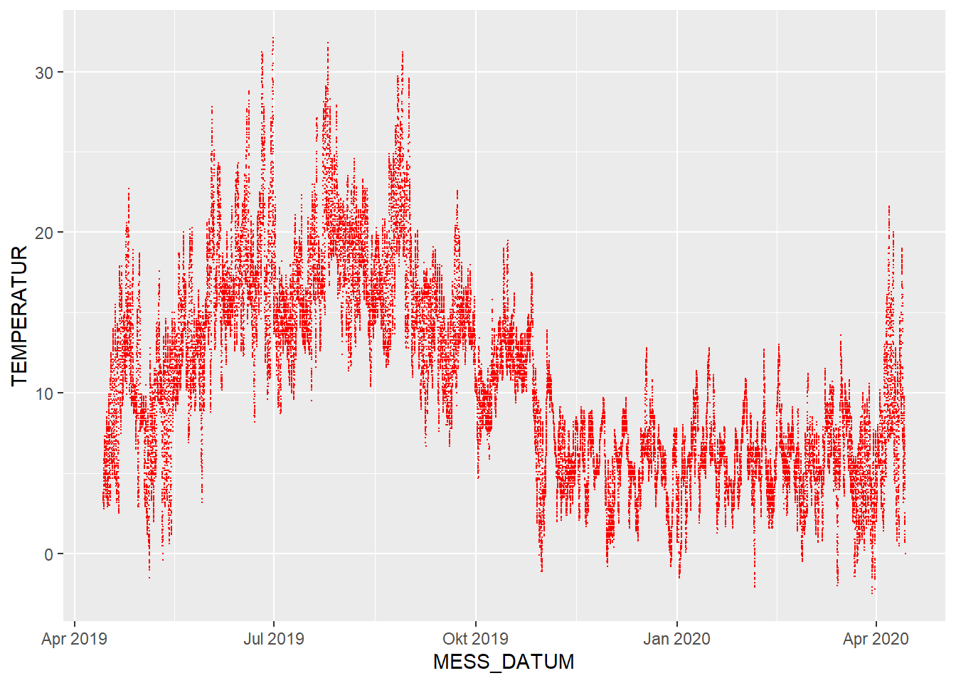 This is a representation of all 52,704 observations of temperature and naturally appears quite crowded.
However, a typical course of the seasons during a year can already be interpreted from this plot.
Please note that the chart starts at the start of the observations (April 2019) and stretches over a year from there.
This is a representation of all 52,704 observations of temperature and naturally appears quite crowded.
However, a typical course of the seasons during a year can already be interpreted from this plot.
Please note that the chart starts at the start of the observations (April 2019) and stretches over a year from there.
Let’S try to get a clearer picture of the temperature variable during the course of the observed year. We need to form averages and aggregates to make visualisation more to the point and get less crowded pictures.
New variables should represent other dimensions of date-time data. We can use lubridate functions to produce variables for hours, 24hdays, weeks, months and even possibly seasons.
Assigning a year to every observation by creating a new column with lubridate function “year”:
Assigning the specific month (number) to every observation by creating a new column with lubridate function “month”
Assigning an Epiweeknr (EKW = Epi Kalender Woche) to every observation through a column with the function “epiweek”:
Assigning a daynumber to every observation by creating a new column “JTAG” (Year day):
Assigning an hour to every observation by creating a new column “STUNDE”:
Our data frame (df) has 12 variables now and thus we can filter the data by year, month, week, day and hour of the day. This gives us new possibilities to aggregate.
The following GROUP_BY command creates a unique grouping per hour and then calculates the average temperature for every hour, then pastes this value into each observation per hour.
df_group_Stunde <- df %>%
  group_by(STATIONS_ID, JAHR, MONAT, EKW, JTAG, STUNDE)

df_av_temp_Stunde  <- df_group_Stunde %>%
  summarise(AVGTEMPH = mean(TEMPERATUR)) %>%
  arrange(STATIONS_ID, JAHR, MONAT, EKW, JTAG, STUNDE)
This newly created table has reduced the number of observations by the factor 6 to 8,784 and reveals the average temperature per hour.
Let’s plot the data again as hourly temperature averages per day:
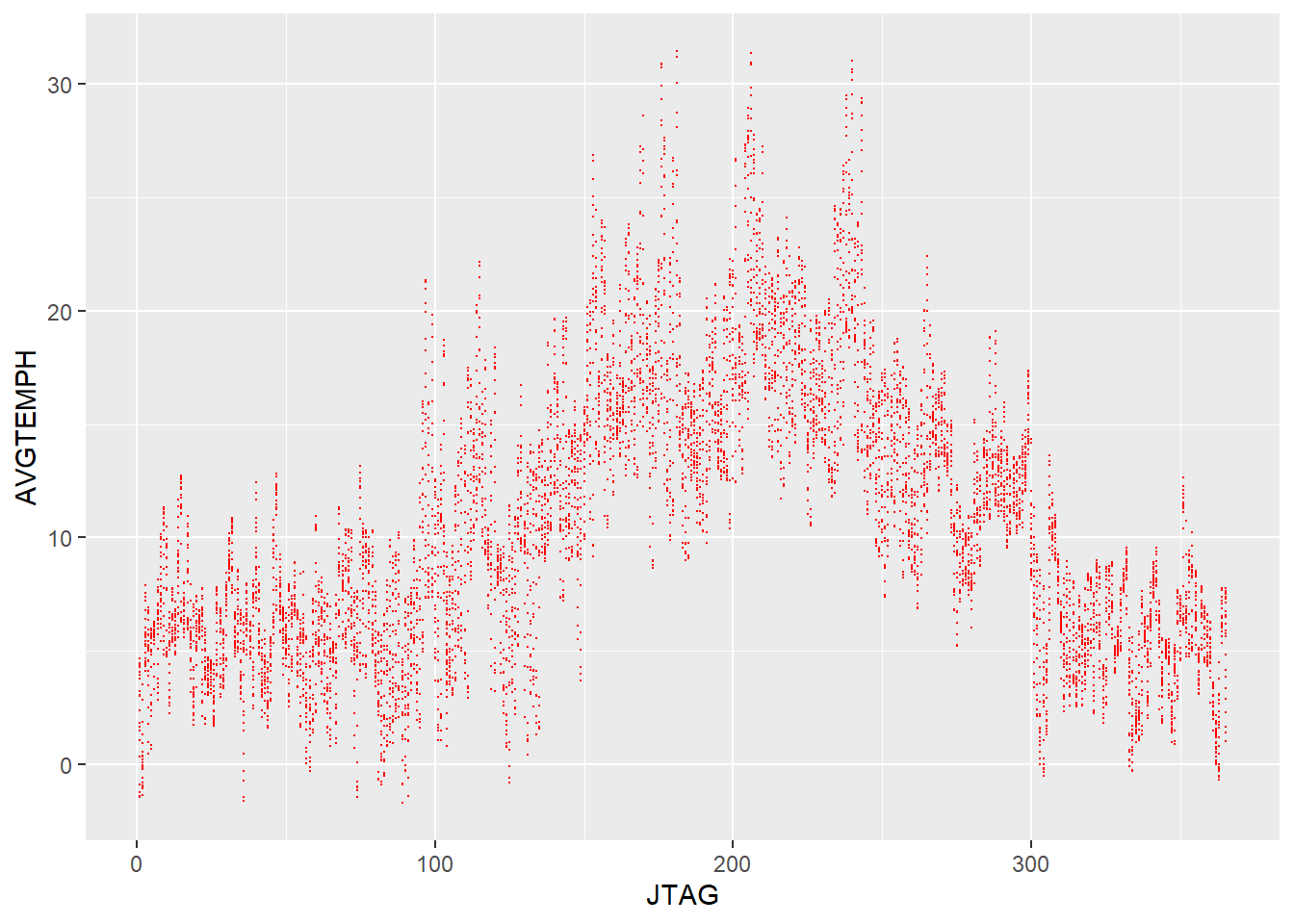 We can see that the data has become aggregated and that the temperature picture becomes somewhat more clear.
Also the visualisation now stretches over the course of a whole calendar year from left to right.
Let’s go one step further and shorten the data down to daily averages by:
We can see that the data has become aggregated and that the temperature picture becomes somewhat more clear.
Also the visualisation now stretches over the course of a whole calendar year from left to right.
Let’s go one step further and shorten the data down to daily averages by:
df_group_JTAG <- df %>%
  group_by(STATIONS_ID, JAHR, MONAT, EKW, JTAG)

df_av_temp_JTAG  <- df_group_JTAG %>%
  summarise(AVGTEMPD = mean(TEMPERATUR)) %>%
  arrange(STATIONS_ID, JAHR, MONAT, EKW, JTAG)
head(df_av_temp_JTAG, 10)
## # A tibble: 10 x 6
## # Groups: STATIONS_ID, JAHR, MONAT, EKW [2]
## STATIONS_ID JAHR MONAT EKW JTAG AVGTEMPD
## <int> <dbl> <dbl> <dbl> <dbl> <dbl>
## 1 2564 2019 4 16 104 4.96
## 2 2564 2019 4 16 105 5.58
## 3 2564 2019 4 16 106 6.43
## 4 2564 2019 4 16 107 8.17
## 5 2564 2019 4 16 108 9.25
## 6 2564 2019 4 16 109 9.63
## 7 2564 2019 4 16 110 8.91
## 8 2564 2019 4 17 111 11.4
## 9 2564 2019 4 17 112 12.2
## 10 2564 2019 4 17 113 12.6This newly created table has reduced the number of observations by the factor 24 to 366 (the number of days in a leap year) and reveals the average temperature per day. Let’s plot the data again as dayly temperature averages over the whole period as a line:
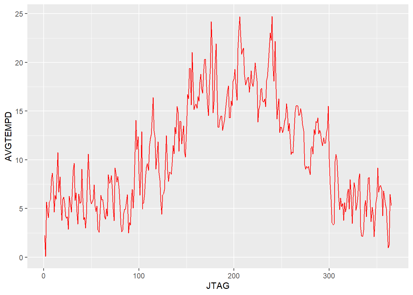 The data starts to make even more visual sense. The key take-aways from this plot, next to the rather trivial finding of higher summer temperatures, is the rather high volatility that appears to be attached to daily average temperature throughout the year. This could be interpreted as the changes between high and low pressure weather systems that cross northern Germany.
Let’s boil the data down to weekly temperature averages:
df_group_EKW <- df %>%
  group_by(STATIONS_ID, JAHR, MONAT, EKW)

df_av_temp_EKW  <- df_group_EKW %>%
  summarise(AVGTEMPW = mean(TEMPERATUR)) %>%
  arrange(STATIONS_ID, JAHR, MONAT, EKW)
head(df_av_temp_EKW, 10)
## # A tibble: 10 x 5
## # Groups: STATIONS_ID, JAHR, MONAT [3]
## STATIONS_ID JAHR MONAT EKW AVGTEMPW
## <int> <dbl> <dbl> <dbl> <dbl>
## 1 2564 2019 4 16 7.56
## 2 2564 2019 4 17 13.2
## 3 2564 2019 4 18 10.4
## 4 2564 2019 5 18 6.66
## 5 2564 2019 5 19 8.43
## 6 2564 2019 5 20 10.2
## 7 2564 2019 5 21 13.4
## 8 2564 2019 5 22 12.9
## 9 2564 2019 6 22 16.3
## 10 2564 2019 6 23 17.7and plot again:
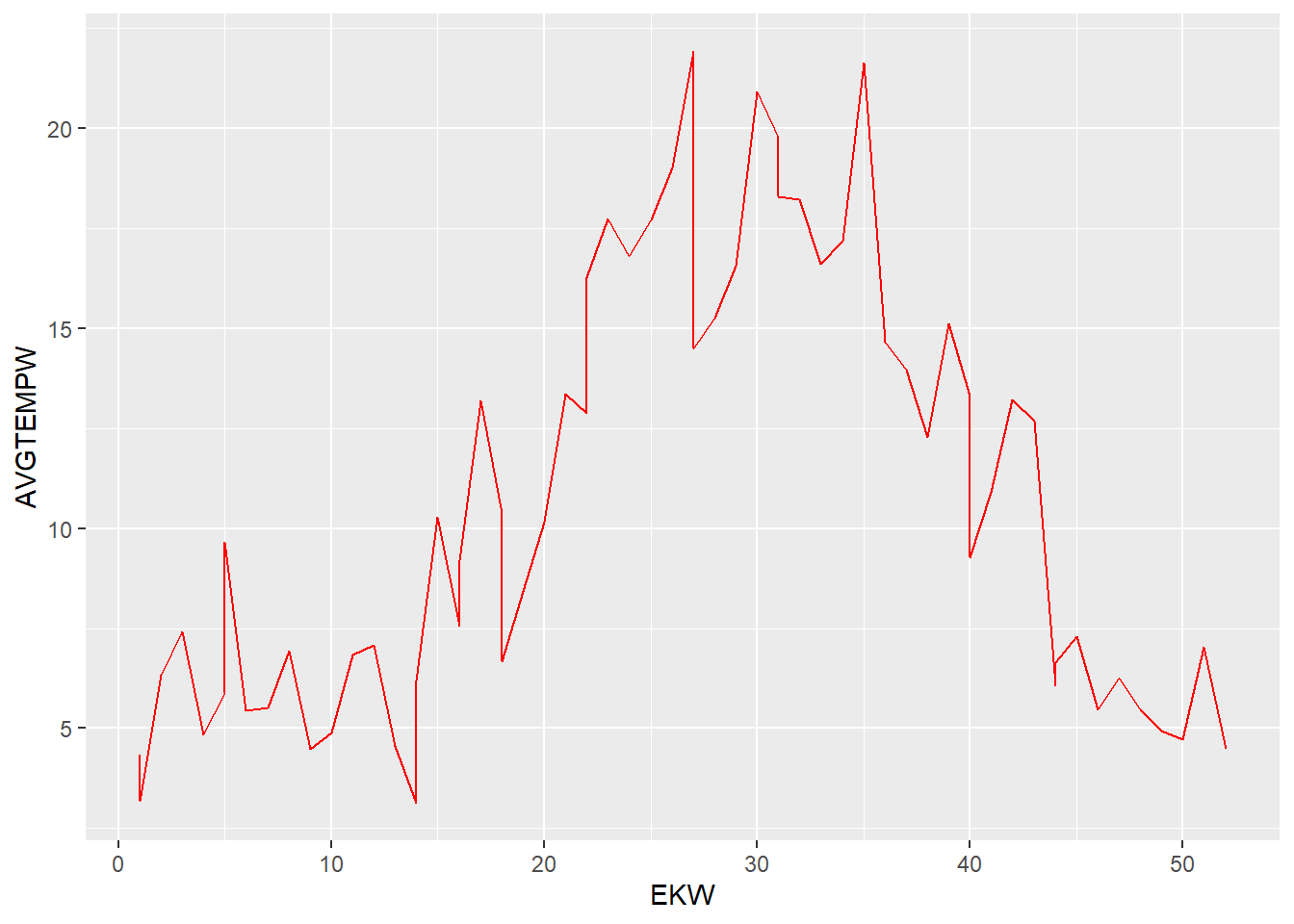 Even in weekyl aggregates of temperature averages the resulting visualisation still tells a story of volatility.
Let’s look at monthly averages:
Even in weekyl aggregates of temperature averages the resulting visualisation still tells a story of volatility.
Let’s look at monthly averages:
df_group_MONAT <- df %>%
  group_by(STATIONS_ID, JAHR, MONAT)

df_av_temp_MONAT  <- df_group_MONAT %>%
  summarise(AVGTEMPM = mean(TEMPERATUR)) %>%
  arrange(STATIONS_ID, JAHR, MONAT)
head(df_av_temp_MONAT, 12)
## # A tibble: 12 x 4
## # Groups: STATIONS_ID, JAHR [2]
## STATIONS_ID JAHR MONAT AVGTEMPM
## <int> <dbl> <dbl> <dbl>
## 1 2564 2019 4 10.4
## 2 2564 2019 5 10.6
## 3 2564 2019 6 17.9
## 4 2564 2019 7 17.3
## 5 2564 2019 8 18.4
## 6 2564 2019 9 14.0
## 7 2564 2019 10 10.8
## 8 2564 2019 11 6.16
## 9 2564 2019 12 5.20
## 10 2564 2020 1 5.74
## 11 2564 2020 2 5.74
## 12 2564 2020 3 5.58and plot again:
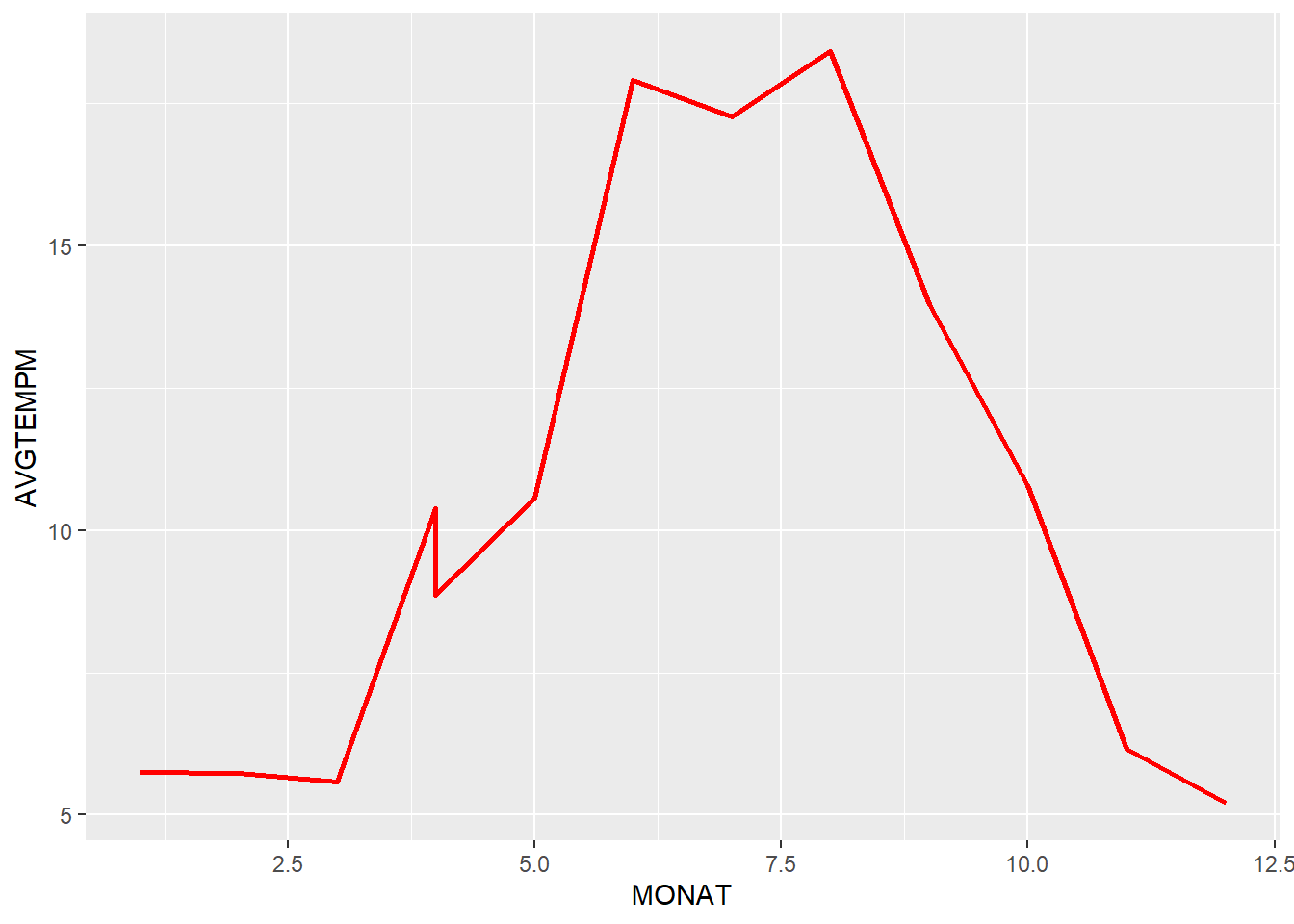 Which is the kind of temperature curve we would expect to see in a north German location like Kiel with a clear pattern of 3 months of summer with higher average temperatures just below 20 degrees.
It is interesting to note that (at least the first half of April 2020 is apparently much warmer on average than the second half of April in 2019. The dimension indicates a difference of about 2 degrees celsius, a significant difference.
4.6.1.1 Average temperature for a day
Generally, no separate variables would have to be created to determine the average temperatures. The values can be gleaned differently from the data frame.
df_avg1 <- df_group %>%
  summarise(avg = mean(TEMPERATUR)) %>%
  arrange( STATIONS_ID , TAG , STUNDE)
head(df_avg1, 10)
## # A tibble: 10 x 4
## # Groups: STATIONS_ID, STUNDE [10]
## STATIONS_ID STUNDE TAG avg
## <int> <int> <int> <dbl>
## 1 2564 0 1 5.45
## 2 2564 1 1 5.32
## 3 2564 2 1 5.22
## 4 2564 3 1 5.3
## 5 2564 4 1 5.53
## 6 2564 5 1 5.58
## 7 2564 6 1 5.35
## 8 2564 7 1 5.9
## 9 2564 8 1 6.18
## 10 2564 9 1 6.54.6.2 Rainfall
4.6.2.1 Sum with condition
The question here is, how long has ist rained during an hour/day? There are two different possible aproaches. One is without the binary indicator and the other uses it as a switch.
Without indicator
df_sum1 <- df_group %>%
  summarise(sum(NIEDERSCHLAGSDAUER)) %>%
  arrange( STATIONS_ID , TAG, STUNDE)
head(df_sum1, 24)
## # A tibble: 24 x 4
## # Groups: STATIONS_ID, STUNDE [24]
## STATIONS_ID STUNDE TAG `sum(NIEDERSCHLAGSDAUER)`
## <int> <int> <int> <int>
## 1 2564 0 1 0
## 2 2564 1 1 0
## 3 2564 2 1 0
## 4 2564 3 1 0
## 5 2564 4 1 0
## 6 2564 5 1 0
## 7 2564 6 1 0
## 8 2564 7 1 0
## 9 2564 8 1 0
## 10 2564 9 1 0
## # ... with 14 more rowsWith indicator and renamed column
df_sum2 <- df_group %>%
  summarise(MENGE = sum(NIEDERSCHLAGSDAUER[NIEDERSCHLAGSINDIKATOR==1])) %>%
  arrange( STATIONS_ID , TAG, STUNDE)
head(df_sum2, 24)
## # A tibble: 24 x 4
## # Groups: STATIONS_ID, STUNDE [24]
## STATIONS_ID STUNDE TAG MENGE
## <int> <int> <int> <int>
## 1 2564 0 1 0
## 2 2564 1 1 0
## 3 2564 2 1 0
## 4 2564 3 1 0
## 5 2564 4 1 0
## 6 2564 5 1 0
## 7 2564 6 1 0
## 8 2564 7 1 0
## 9 2564 8 1 0
## 10 2564 9 1 0
## # ... with 14 more rowsNow we apply the knowledge with the indicator to the selection of autumn. Now we examine the duration of rainfall in autumn.
df_sum_autmn <- df_group_autmn %>%
  summarise(DAUER = sum(NIEDERSCHLAGSDAUER[NIEDERSCHLAGSINDIKATOR==1])) %>%
  arrange( STATIONS_ID , JAHR, MONAT, TAG)
head(df_sum_autmn, 10)
## # A tibble: 10 x 5
## # Groups: STATIONS_ID, TAG, MONAT [10]
## STATIONS_ID TAG MONAT JAHR DAUER
## <int> <int> <dbl> <dbl> <int>
## 1 2564 23 9 2019 0
## 2 2564 24 9 2019 11
## 3 2564 25 9 2019 593
## 4 2564 26 9 2019 181
## 5 2564 27 9 2019 392
## 6 2564 28 9 2019 228
## 7 2564 29 9 2019 1008
## 8 2564 30 9 2019 354
## 9 2564 1 10 2019 752
## 10 2564 2 10 2019 1464.6.3 Humidity
What we can say at this point is that the temperatures in the city of Kiel have a clear seasonal pattern, but remain highly volatile intra-day and inter-day.
Weather however is not just defined as temperature, but humidity and precipitation play a role regarding our sensation and definition of weather as well.
Let’s have one look at humidity the same way we looked at temperatures as hourly averages:
df_av_humi_Stunde  <- df_group_Stunde %>%
  summarise(AVGHUMI = mean(RELATIVE_FEUCHTE)) %>%
  arrange(STATIONS_ID, JAHR, MONAT, EKW, JTAG, STUNDE)
Let’s plot the data again as hourly humidity averages per day:
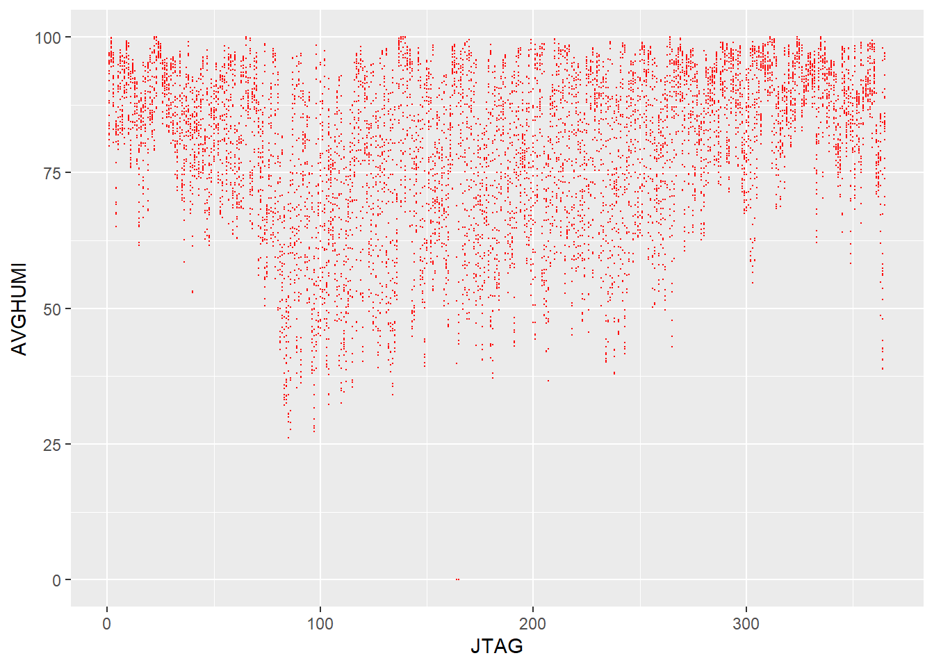 This plot shows the dryer months during the summer as having a lot more hours with lower humidity values than the months that fall into autumn and winter.
4.7 Wrap up
It was our objective to show and explain some of the more important features of the lubridate package. We can definitely say that handling this dataset in Base R would have been a lot more labourious. Lubridate has made working with this time series if not easy, but possible. This statement goes for the other used packages in this exploration (dplyr, ggplot, etc.) without which the whole task would have been quite tedious.